esa_cci_sm
Reading and reshuffling of CCI soil moisture Written in Python.
Installation
Installing the package can be done via pip:
pip install esa_cci_sm
Setup of a complete development environment with conda can be performed using the following commands:
git clone git@github.com:TUW-GEO/esa_cci_sm.git esa_cci_sm
cd esa_cci_sm
conda env create -f environment.yml
source activate esa_cci_sm
Supported Products
At the moment this package supports ESA CCI soil moisture data version v02.x and v03.x and v04.x in netCDF format (reading and time series creation) with a spatial sampling of 0.25 degrees.
Contribute
We are happy if you want to contribute. Please raise an issue explaining what is missing or if you find a bug. We will also gladly accept pull requests against our master branch for new features or bug fixes.
Development setup
For Development we also recommend a conda environment. You can create one
including test dependencies and debugger by running
conda env create -f environment.yml. This will create a new esa_cci_sm
environment which you can activate by using source activate esa_cci_sm.
Guidelines
If you want to contribute please follow these steps:
- Fork the esa_cci_sm repository to your account
- Clone the repository, make sure you use
git clone --recursiveto also get the test data repository. - make a new feature branch from the esa_cci_sm master branch
- Add your feature
- Please include tests for your contributions in one of the test directories. We use py.test so a simple function called test_my_feature is enough
- submit a pull request to our master branch
Note
This project has been set up using PyScaffold 2.5. For details and usage information on PyScaffold see http://pyscaffold.readthedocs.org/.
Reading ESA CCI SM images
Reading of the ESA CCI SM raw netcdf files can be done in two ways.
Reading by file name
import os
from datetime import datetime
from esa_cci_sm.interface import CCI_SM_025Img
import numpy.testing as nptest

# read several parameters
parameter = ['sm', 'sm_uncertainty']
# the class is initialized with the exact filename.
image_path = os.path.join(os.path.dirname(__file__), 'tests', 'esa_cci_sm-test-data',
                          'esa_cci_sm_dailyImages', 'v04.2', 'combined', '2016')
image_file = 'ESACCI-SOILMOISTURE-L3S-SSMV-COMBINED-20160607000000-fv04.2.nc'
img = CCI_SM_025Img(os.path.join(image_path, image_file), parameter=parameter)

# reading returns an image object which contains a data dictionary
# with one array per parameter. The returned data is a global 0.25 degree
# image/array.
image = img.read()
Reading by date
All the ESA CCI SM data in a directory structure can be accessed by date. The filename is automatically built from the given date.
from esa_cci_sm.interface import CCI_SM_025Ds

parameter = 'sm'
img = CCI_SM_025Ds(data_path=os.path.join(os.path.dirname(__file__),
                                                'tests', 'esa_cci_sm-test-data', 'esa_cci_sm_dailyImages',
                                                'v04.2', 'combined'),
                          parameter=parameter)

image = img.read(datetime(2016, 6, 7, 0))
For reading all image between two dates the
c3s_sm.interface.CCI_SM_025Ds.iter_images() iterator can be
used.
Variable names for ESA CCI Soil Moisture
ESA CCI SM variables as in the netcdf image files (and time series from netcdf images) for different products and versions
| short_name | Parameter | Units |
|---|---|---|
| dnflag | Day / Night Flag | |
| flag | Flag | |
| freqbandID* | Frequency Band Identification | |
| lat | Latitude | [degrees_north] |
| lon | Longitude | [degrees_east] |
| mode | Satellite Mode | |
| sensor | Sensor Flag | |
| sm | Volumetric Soil Moisture | [m3 m-3] |
| sm_uncertainty | Volumetric Soil Moisture Uncertainty | [m3 m-3] |
| t0 | Observation Timestamp | [days since 1970-01-01 00:00:00 UTC] |
| time | Time | [days since 1970-01-01 00:00:00 UTC] |
- “freqbandID” is named “freqband” in older versions (before v3) of the data set.
Conversion to time series format
For a lot of applications it is favorable to convert the image based format into a format which is optimized for fast time series retrieval. This is what we often need for e.g. validation studies. This can be done by stacking the images into a netCDF file and choosing the correct chunk sizes or a lot of other methods. We have chosen to do it in the following way:
Store only the reduced gaußian grid points since that saves space.
Further reduction the amount of stored data by saving only land points if selected.
Store the time series in netCDF4 in the Climate and Forecast convention Orthogonal multidimensional array representation
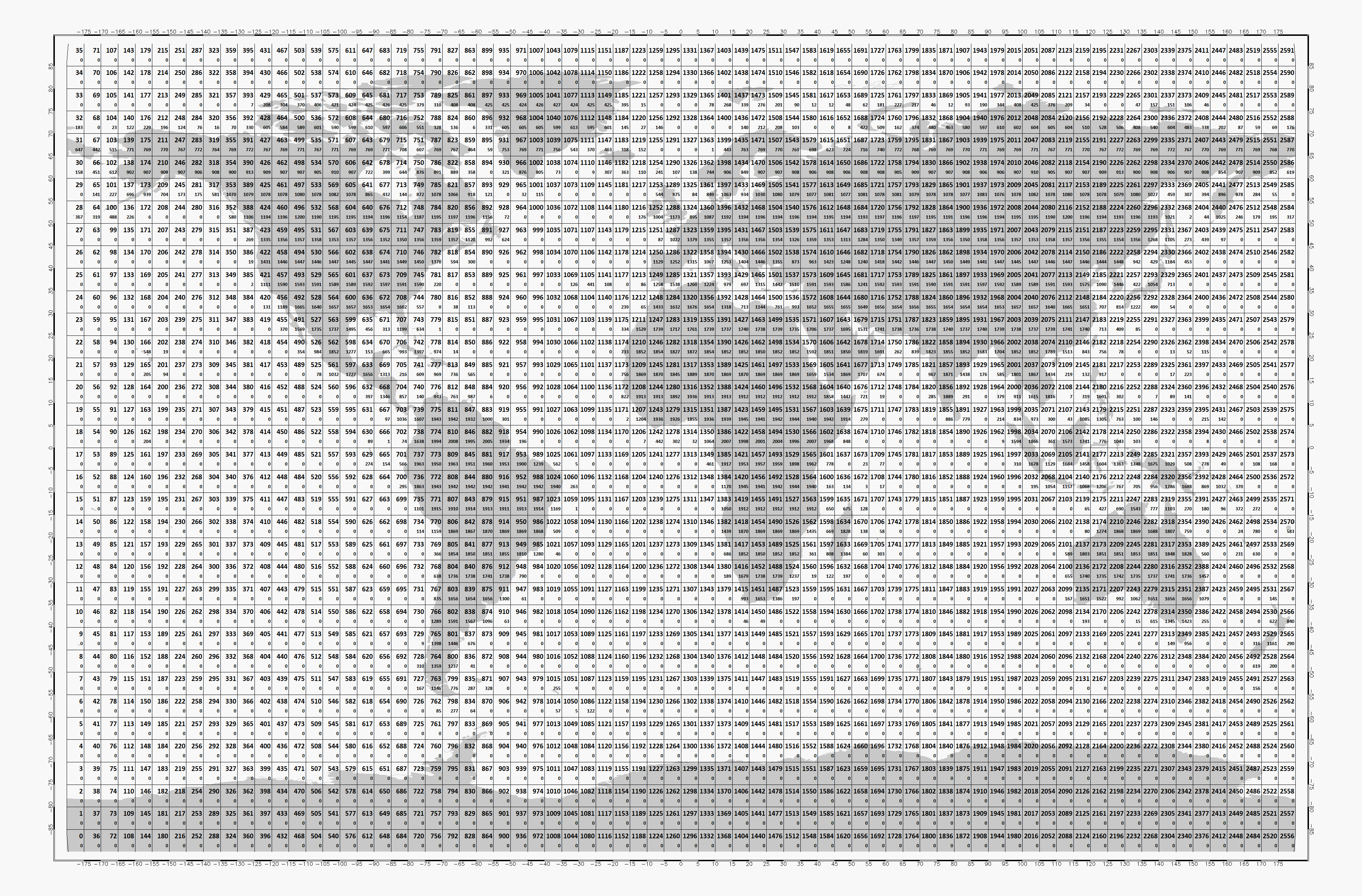
Store the time series in 5x5 degree cells. This means there will be 2566 cell files (1001 with reduction to land points) and a file called
grid.ncwhich contains the information about which grid point is stored in which file. This allows us to read a whole 5x5 degree area into memory and iterate over the time series quickly.
This conversion can be performed using the ccism_reshuffle command line
program. An example would be:
ccism_reshuffle /cci_images /timeseries/data 2000-01-01 2001-01-02 --parameters sm sm_uncertainty --land_points True
Which would take ESA CCI SM data stored in /cci_images over land from January 1st
2000 to January 2nd 2001 and store the parameters for soil moisture and its uncertainty as time
series in the folder /timeseries/data.
Note: If a RuntimeError: NetCDF: Bad chunk sizes. appears during reshuffling, consider downgrading the
netcdf4 C-library via:
conda install -c conda-forge libnetcdf==4.3.3.1 --yes
Conversion to time series is performed by the repurpose package in the background. For custom settings
or other options see the repurpose documentation and the code in
esa_cci_sm.reshuffle.
Reading converted time series data
For reading the data the ccism_reshuffle command produces the class
CCITs can be used:
from esa_cci_sm.interface import CCITs
ds = CCITs(ts_path)
# read_ts takes either lon, lat coordinates or a grid point indices.
# and returns a pandas.DataFrame with all reshuffled variables.
    # e.g. timeseries for lon=45°, lat=15°:
ts = ds.read_ts(45, 15)